I’ve been studying a Computational Finance module for the past few months now, and it’s absolutely fascinating. This blog post focuses on Markowitz Portfolio Optimization (AKA Modern portfolio theory), and will be part of a number of Computational Finance posts I’ll be posting over the coming months. The following post includes MATLAB examples, but these could be adapted to other languages such as Python.
So first of all, some basic definitions.
Definitions
Stock – In this context, a “stock” is a holding in a company that might be traded through the stock market
Portfolio – A collection of financial assets. In this context, I’ll be talking in terms of holdings of financial stocks. So for example, £30 in company A, £70 in company B. For the purposes of this blog post, it is better to think in terms of percentages. In the previous example, that would therefore be 30% in company A and 70% in company B if I had a total portfolio of £100.
Markowitz Portfolio Optimization
Markowitz Portfolio Optimization (modern portfolio theory, MPT for short), is a theory used in the real world to decide on how best to invest your money in a given set of stocks (Markowitz, 1952). It works with two underlying variables: risk and return. It attempts to maximize returns of a portfolio for a given allowable risk, or minimize risk of a portfolio for a selected return. For example, you may say you want a return of 10%, and you want to invest in a selection of, say, 20 stocks. Using some relatively straightforward calculations that we’ll cover, we can find the optimum portfolio (I.E. the proportions for which we invest our money in each stock) in which the risk of losing money is minimized as low as it can be while still reaching our target return.
Sounds useful! We tell it the stocks we’re interested in, and it tells us how much to invest in each one according to our desires risk or our desired return. But how do we define risk and return? In order to do so, we need to define some mathematical variables. Throughout, we’ll assume we’re interested in only three stocks, A B and C.
Variables
w – A vector representing our portfolio weights. I use the term weights here because each element of the vector represents the weighting of investment (out of our total starting money) in a particular stock. For example, if we have stocks A B and C, we might have a w = [0.10 0.50 0.40], which represents an investment of 10% of our money in stock A, 50% in stock B and 40% in stock C.
R – A matrix containing the historical return data of each stock, where each column represents an individual stock, and each row of the column represents the return of that stock at a point in time. Rit is therefore the return on stock i at time t. Conventions differ for how the return is defined, but I will use the proportional change from open price to close price of a particular day for a particular stock. So for example, if Rit = 0.02, then stock i rose by 0.02% on day t.
m – A vector representing the average returns of the individual stocks on historical data over a period of time. This is calculated over a time period, and it is calculated by averaging the proportional change over a time period. For example, we could take the value of stock i at time t = 1, and its value at time t = T, and the percentage change between the two time points would be represented by mi, the mean return of stock i. The m vector is laid out in a similar fashion as w: m = [mA mB mC]. Mathematically, the mean return for stock i over a period from t=1 to t=T is:

We can perform this calculation in MATLAB like so:
% Ntraining = number of samples to use in training w
% R = historic stock data samples
mean( R(1:Ntraining, :) );
C – A matrix representing the covariances (AKA covariance matrix) between all of the stocks, calculated from historical data over a period of time. If you’re unfamiliar with covariance matrices or you need a refresher, here is a good online resource. While the formulation of such a matrix is not important to remember since it can be easily calculated using MATLAB or other tools, it is important to understand the significance of the covariance matrix in this context. Put simply, the covariance is a measure of the correlation[note]Technically, it’s not the statistical correlation of two variables, but it is a measure of how much they “move together”. It is basically statistical correlation, only it is not scaled to lie within the range -1 and 1. This is not a problem, however, as we are not comparing two different sets of stocks, just A B and C. If we wanted to see how stock A and stock B correlated compared to stock D and stock E in a different data set, we would need to calculate the statistical correlation[/note] between two variables. If two variables go up over time, they have a positive covariance. If one variable goes up and the other goes down, they have a negative covariance. In this context, the covariance matrix represents the correlations between stocks A B and C. One could say that element Cij is a measure of how stock j correlates with stock i. C is symmetrical, since the correlation of stock j with stock i is the same as the correlation of stock i with stock j, I.E. Cij = Cji. The diagonal of the matrix, I.E. when i = j, is the variance of each stock. The variance of a stock can be thought of as how “risky” that stock is. If it fluctuates a lot, we might consider it risky to invest in it. We’ll come back to this assumption later. If this all seems a bit confusing, that’s okay. Just remember that C is a variable that stores the correlation between each stock (A and B, A and C, B and C) and the variances of each stock (A B and C).
We can perform the calculation of C in MATLAB like so:
% Ntraining = number of samples to use in training w
% R = historic stock data samples
cov( R(1:Ntraining, :) );
Defining Risk and Return
Now that we have some underlying definitions and variables to use, we can define what exactly risk and return are.
Firstly, it is helpful to point out a relationship between the returns of a stock, R, and the returns of a portfolio. The returns of a portfolio is defined as ρ, and it is mathematically defined as:

The resulting ρ is a vector in which each row represents the returns of that particular day, given the weighting of investment of each stock. For the purposes of MPT, all we need to know is that ρ is a linear transform of R.
Secondly, we need to make an assumption about how we model the returns R when estimating future expected values of returns. It’s all well and good having historic data, but how do we extrapolate to estimate what R might do in the future? The returns R are modelled as multivariate Gaussian distributions. We write the Gaussian distribution of R as :
")
Where:


We also use the following relationship:
")
Using this relationship, and the relationship in (1), we have:
")
Substituting mean and variance:
")
Still with me? If so, the rest will be a breeze. If you didn’t quite understand the derivation above, don’t worry too much. Just make sure that you understand the two meaningful terms we obtained, return and risk, from the above equation:


Representing the Problem Mathematically
So, now we finally have a way to calculate return and risk of a portfolio. We base these calculations on historic data (represented in m and C). But, historic data is not immediately useful. What good is it that we can plug in different numbers into our portfolio w and have it tell us what we would have got had we invested this portfolio? Rather than saying “Here’s a portfolio, go and figure out what I get in terms of return and risk“, we really want to be able to say “Give me a portfolio that will give me x return, but has the least possible risk“. That sounds like it might be complicated, but this sort of problem is actually just a straightforward optimization problem! We can write this mathematically, using our little formulas for risk and return above:

For those unfamiliar with optimization problems, this simply says “Find the portfolio weights, w, with the minimum possible risk that gives me return r0“. The good thing about this minimization equation is that we’ve now got a succinct mathematical way of representing exactly what we said in words before. There are many mathematical tools out there that can compute such problems, and below is an example using the CVX toolbox for MATLAB which performs the minimization problem. CVX is nice because it has an intuitive interface which is quite similar to the mathematical representation.
cvx_begin
    variable w(N) % N = number of assets
        minimize(w'*C*w)
        subject to
            w'*ones(N, 1) == 1,
            w'*m == r0,
            w > 0;
cvx_end
The first constraint in the above code ensures that the elements in w add up to 1 (100%). Of course, we cannot have 110% of our money invested in a portfolio, and we also would not want only 90% of it invested, for example. The second constraint is the constraint we’re already familiar with, the part that states that we must obtain the return we’re seeking, r0. The final constraint ensures that all of the elements of w are positive. This constraint imposes a limit of no “short-selling”.
So, what is the result? Running the above code gives us some weights in w, representing the portfolio which would give you the lowest possible risk while still giving you your desired return r0. That’s pretty neat! Of course, C and m are calculated on historic stock data, and since we’re actually interested in applying the resulting portfolio to futuristic data (I.E. we want to invest our portfolio now and see its performance after some time has passed), we’re working under the assumption that the stock’s risks and mean returns (C and m) are representative of how the stocks will behave in future, based on their past. So the resulting weights are obviously only really “estimations” of the optimum portfolio when applied to future investments. We call the historic stock data “training data”, because we’re using it to “train” w. We can actually also use some more historic data that hasn’t been used in the calculation of C and m in order to see how the portfolio performs in “real-world” scenarios. This data we use to test the performance is called “test data”, because we’re using it to verify the returns of w on data that it hasn’t been trained on. It is still historic data, but it allows us to see how our portfolio would have performed on some “unseen” data. In other words, it allows us to see how the portfolio would have performed if we had actually invested in the proportions given by w. Of course, we could indeed invest in these proportions, and see how the portfolio performs, but it is clearly more efficient to simply emulate this by pretending some historic data is what we’re investing on.
There’s another way we could approach optimizing our portfolio which I mentioned at the start. Rather than seeking the portfolio that gives us the lowest risk for a particular desired return, we can instead seek the portfolio which gives us the highest return for a maximum risk limit. Mathematically, we can write this as such:

Similarly to before, this formula simply states “Find the portfolio weights, w, that give me the maximum possible return that has a risk of σ0“. Again, numerous mathematical tools exist to solve this kind of optimization problem. The code for CVX is as follows:
cvx_begin
    variable w(N) % N = number of assets
        maximize(w'*m)
        subject to
            w'*ones(N, 1) == 1,
            w'*C*w == s0,
            w > 0;
cvx_end
This code is very similar to the previous approach, only the risk and return terms have been swapped, and the risk constraint is s0 (σ0). Think about what might happen if we removed the risk constraint. If you want to know the answer, hover over this footnote[note]The maximization would simply result in a portfolio in which 100% of the money is invested in the stock which simply gives the best return, but not necessarily the least risky, as it would clearly not even consider risk![/note].
Efficient Frontier
Hopefully you’re still with me by this point. So far, we’ve calculated two different portfolios: one in which we want to minimize risk for a given return, and one where we want to maximize return for a given risk. This is all well and good, but clearly there are some limits to what we can choose for our risk or return constraints. For example, we can’t choose to have a 200% return and expect a portfolio to be able to achieve that, no matter what risk we allow. Likewise, how do we choose a sensible limit for risk, especially since it’s dimensionless? This is where something called the Efficient Frontier comes in. The Efficient Frontier is a characteristic we can calculate and plot which demonstrates, for a particular selection of stocks, what the best possible trade off between risk and return is. An example of an Efficient Frontier is shown in Figure 1.
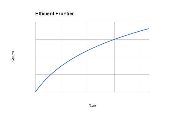
Figure 1 – Efficient Frontier example
This demonstrates the maximum realizable returns for a range of risks. We can see that, as we increase our risk, we can obtain better returns – which intuitively makes sense. The Efficient Frontier, represented by the blue line, represents the most efficient trade-off between risk and return possible for a particular selection of stocks. All of the points on the line represent the maximum possible realizable returns for their corresponding risks. Of course, we cannot select a point above the line (I.E. we cannot seek a return greater than the point on the Efficient Frontier for a given risk). We could indeed select a point below the line (I.E. accept a lower return for the same risk), but this is inefficient. So, in order to find some sensible values to plug into our calculations in the MATLAB code above, we can plot the Efficient Frontier, choose a good trade-off between risk and return by selecting a point on the line, and plug the value of risk in to our code above by setting s0 to it.
But how do we calculate the Efficient Frontier? The steps are outlined below.
- Find the portfolio with the maximum possible return, unconstrained by risk
- Calculate the risk of this portfolio, this will be the maximum possible risk
- Find the portfolio with the minimum possible risk, unconstrained by return
- The risk of this portfolio will be the minimum possible risk
- Make a list of risks by stepping from the least possible risk calculated in step 2, up to the risk calculated in 1 and incrementing in small steps, forming our x axis
- Using each risk in the list as a constraint, calculate the portfolio with the maximum possible return for each risk
The MATLAB code to perform this is shown below. The code is adapted from (Brandimarte, 2006), but I have replaced equivalent parts with CVX code since that’s what we’re now familiar with.
function [PRisk, PRoR, PWts] = NaiveMVCVX(ERet, ECov, NPts)
    ERet = ERet(:); % makes sure it is a column vector
    NAssets = length(ERet); % get number of assets
    % vector of lower bounds on weights
    V0 = zeros(NAssets, 1);
    % row vector of ones
    V1 = ones(1, NAssets);
    % Find the maximum expected return
    cvx_begin
    variable w(NAssets)
        maximize(w'*ERet)
        subject to
            w'*ones(NAssets, 1) == 1;
            w > 0;
    cvx_end
    MaxReturnWeights = w
    MaxReturn = MaxReturnWeights' * ERet;
    % Find the minimum variance return
    cvx_begin
    variable w(NAssets)
        minimize(w'*ECov*w)
        subject to
            w'*ones(NAssets, 1) == 1,
            w > 0;
    cvx_end
    MinVarWeights = w
    MinVarReturn = MinVarWeights' * ERet;
    MinVarStd = sqrt(MinVarWeights' * ECov * MinVarWeights);
    % check if there is only one efficient portfolio
    if MaxReturn > MinVarReturn
        RTarget = linspace(MinVarReturn, MaxReturn, NPts);
        NumFrontPoints = NPts;
    else
        RTarget = MaxReturn;
        NumFrontPoints = 1;
    end
    % Store first portfolio
    PRoR = zeros(NumFrontPoints, 1);
    PRisk = zeros(NumFrontPoints, 1);
    PWts = zeros(NumFrontPoints, NAssets);
    PRoR(1) = MinVarReturn;
    PRisk(1) = MinVarStd;
    PWts(1,:) = MinVarWeights(:)';
    % trace frontier by changing target return
    VConstr = ERet';
    A = [V1 ; VConstr ];
    B = [1 ; 0];
    for point = 2:NumFrontPoints
        B(2) = RTarget(point);
        cvx_begin quiet
            variable w(NAssets)
                minimize(w'*ECov*w)
                subject to
                    w'*ones(NAssets, 1) == 1,
                    w'*ERet == RTarget(point), %this time we're targeting RTarget
                    w >= 0;
        cvx_end
        Weights = w;
        PRoR(point) = dot(Weights, ERet);
        PRisk(point) = sqrt(Weights'*ECov*Weights);
        PWts(point, :) = Weights(:)';
    end
end
Alternatively, if you have access to the financial toolbox, you can use the MATLAB function frontcon to calculate the efficient frontier for you. The two approaches give identical results, but frontcon is faster.
You could, as mentioned previously, simply pick a desirable risk from the Efficient Frontier and use the weights associated with it. Alternatively, you could use the Sharpe ratio to determine the optimum trade off between risk and return by calculating the Sharpe ratio for each portfolio that exists on the efficient frontier. The Sharpe ratio (Sharpe, 1994) is defined as:

rp– portfolio return.
rf – risk-free return. This is the return we’d get if we instead just dumped all the money in the portfolio into a bank where the interest rate is constant and you can never really lose. Set this to 0 if you’re not interested in investing in such a manner. Otherwise, you can include the return you’d get in the original matrix R.
σp– portfolio risk.
The optimum portfolio out of all the portfolios calculated on the Efficient Frontier is the one which gives the largest Sharpe ratio. Simply iterate over the elements in the efficient frontier, calculate the return for each, and pick accordingly, like so:
%calculate the efficient frontier
[risk, returns, w] = frontcon(m, C, 100);

%calculate Sharpe ratio on the training data, and extract the best
%performing portfolio
for i=1:length(returns),
    sharpeTrainingRatios(i) = returns(i)/risk(i);
end

%extract the most efficient portfolio
[maxSharpeTrainingRatio, maxSharpeTrainingRatioIndex] = max(sharpeTrainingRatios);
efficientPortfolio = w(maxSharpeTrainingRatioIndex, :);
Recap
We saw the foundations and assumptions that MPT is based upon, the goals for optimizing a portfolio, and the formulas for calculating risk and return. We saw how to use these formulas to derive optimization problems that we can express programmatically to obtain an optimized portfolio. Finally, we saw how to find the best trade-off for a set of portfolios using the Efficient Frontier and the Sharpe ratio. Now it’s up to you to go and implement these tools, and see for yourself if you can make a good investment!
References
Markowitz, H. (1952). Portfolio Selection. The Journal of Finance, 7(1), p.77.
Brandimarte, P. (2006). Numerical methods in finance and economics. Hoboken, N.J.: Wiley Interscience.
Sharpe, W. (1994). The Sharpe Ratio. The Journal of Portfolio Management, 21(1), pp.49-58.
Leave a Reply